Table of contents
Open Table of contents
概要
注意: この記事は LLM を用いて執筆を補助しており、内容の正確性を保証するものではありません。誤りを見つけた場合はご指摘いただけると助かります。
準モンテカルロ法について自分用にまとめた記事です。 ベイズ最適化の初期点として準モンテカルロ法で用いられている点列(例 Sobol sequence)が使われていることは知っていましたが、具体的にどういうものなのか分かっていなかったので整理した形です。
準モンテカルロ法の背景
各軸を
モンテカルロ積分は
等間隔格子法では同じ精度を達成するために必要な点の数が
まず平均について、
となり、
3行目では独立性から交差項
次元の呪いはモンテカルロ法で解決できましたが、標準誤差が
準モンテカルロ法
準モンテカルロ法は、乱数の代わりに low-discrepancy sequence(LDS) を用いた数値積分方法です。
主な用途は以下の通りです。
次に、点列の一様性を測る指標である discrepancy を定義し、discrepancy と積分誤差を結びつける Koksma-Hlawka の不等式を紹介します。その後、discrepancy が小さい具体的な点列(LDS)を見ていきます。
Discrepancy
モンテカルロ法では一様乱数を扱いますが、乱数の代わりに
直感的には、discrepancy は点列が
ここで
の集合です。
実用上よく使われるのは star-discrepancy
ここで
Low-discrepancy sequence とは、
Koksma-Hlawka の不等式
Discrepancy が積分誤差とどう関係するのかを示すのが Koksma-Hlawka の不等式です 4。
この不等式は、積分誤差が 関数の複雑さ
後述する具体的な LDS(van der Corput, Halton, Sobol など)については
次元
それにもかかわらず、実用上は高次元でも QMC がモンテカルロ法を大幅に上回ることが経験的に知られています。
例えば Paskov と Traub 1 は
Low-discrepancy sequence の具体例
以下では、具体的な LDS の例を紹介します。
Van der Corput sequence 6
具体的に数式で表してみましょう。
正の整数
となります。ここで全ての
で表されます。
この式の定義があまり直感的でないと思う人は次のように考えても良いと思います。
| 整数 | 逆 | 10進表記 | |
|---|---|---|---|
| 1 | 1 | 0.1 | 0.5 |
| 2 | 10 | 0.01 | 0.25 |
| 3 | 11 | 0.11 | 0.75 |
| 4 | 100 | 0.001 | 0.125 |
| 5 | 101 | 0.101 | 0.625 |
| 6 | 110 | 0.011 | 0.375 |
| 7 | 111 | 0.111 | 0.875 |
このテーブルの一番右の列の値が van der Corput sequence に対応します。
van der Corput sequence の最初の
数値シミュレーションをしてみましょう。
コード
import jax; jax.config.update("jax_enable_x64", True)
import jax.numpy as jnp
import numpy as np
import matplotlib.pyplot as plt
from sympy.ntheory.factor_ import totient

def van_der_corput(n: int, b: int):
    x = 0
    inv_b = 1.0 / b
    while n > 0:
        x += (n % b) * inv_b
        n //= b
        inv_b /= b

    return x

def van_der_corput_seq(n: int, b: int) -> jnp.ndarray:
    return jnp.array([van_der_corput(_n, b) for _n in range(n)])

base = 10
N = int(3e2)
n_list = range(N)
seq = van_der_corput_seq(N, base)

fig, ax = plt.subplots(figsize=(6, 6), tight_layout=True)
for n in n_list:
    # Note: 縦軸の n に応じて今までに得られた数列 seq[:n] をプロットしている
    s = seq[:n]
    ax.scatter(s, [n] * len(s), s=1, c='royalblue', alpha=0.2)
ax.set_ylabel(r'$n$')
ax.set_xlabel(r'$x_n$')
ax.set_xlim([0, 1])
ax.set_ylim([0, N])
ax.invert_yaxis()
ax.set_title('Van der Corput sequence (base 10)')
plt.show()
上図より、
積分誤差の比較: モンテカルロ vs QMC (van der Corput)
テスト関数
コード
from functools import partial

import jax
import jax.lax as lax

jax.config.update("jax_enable_x64", True)
import jax.numpy as jnp
import jax.random as jr
import matplotlib.pyplot as plt


def van_der_corput(n: int, b: int):
    x = 0
    inv_b = 1.0 / b
    while n > 0:
        x += (n % b) * inv_b
        n //= b
        inv_b /= b

    return x


def van_der_corput_jax(n, b: int) -> jnp.ndarray:
    """`van_der_corput` と同じ更新式。スカラー n 用(vmap / jit 可能)。"""
    inv_b0 = jnp.float64(1.0 / b)

    def cond(state):
        n_curr, _, _ = state
        return n_curr > 0

    def body(state):
        n_curr, x, inv_b = state
        digit = jnp.mod(n_curr, b)
        x = x + inv_b * digit.astype(jnp.float64)
        n_curr = n_curr // b
        inv_b = inv_b / jnp.float64(b)
        return (n_curr, x, inv_b)

    n0 = jnp.asarray(n, dtype=jnp.int64)
    _, x_out, _ = lax.while_loop(cond, body, (n0, jnp.float64(0.0), inv_b0))
    return x_out


def van_der_corput_seq(n: int, b: int) -> jnp.ndarray:
    return jnp.array([van_der_corput(_n, b) for _n in range(n)])


@partial(jax.jit, static_argnums=(0, 1))
def van_der_corput_seq_jax(n: int, b: int) -> jnp.ndarray:
    """0..n-1 を van der Corput で変換。`van_der_corput_jax` (= `van_der_corput` と同算法) を vmap。"""
    ks = jnp.arange(n, dtype=jnp.int64)
    return jax.vmap(lambda k: van_der_corput_jax(k, b))(ks)


def van_der_corput_base2_seq(n: int) -> jnp.ndarray:
    return van_der_corput_seq_jax(n, 2)


true_value = jnp.e - 1  # ∫₀¹ eˣ dx = e - 1

N_list = jnp.unique(jnp.logspace(1, 4, 80).astype(int))
n_mc_trials = 50  # モンテカルロの試行回数
mc_master_key = jr.PRNGKey(0)

qmc_errors = []
mc_errors_mean = []

for N in N_list:
    N = int(N)
    # QMC (van der Corput, base 2)
    pts_qmc = van_der_corput_base2_seq(N)
    qmc_est = jnp.mean(jnp.exp(pts_qmc))
    qmc_errors.append(float(jnp.abs(qmc_est - true_value)))

    # Monte Carlo (複数試行を一度にサンプル)
    mc_keys = jr.split(mc_master_key, n_mc_trials + 1)[1:]
    pts_mc = jax.vmap(lambda k: jr.uniform(k, (N,), dtype=jnp.float64))(mc_keys)
    mc_est = jnp.mean(jnp.exp(pts_mc), axis=1)
    mc_errors_mean.append(float(jnp.mean(jnp.abs(mc_est - true_value))))

fig, ax = plt.subplots(figsize=(7, 5), tight_layout=True)

ax.loglog(N_list, mc_errors_mean, "o", color="salmon", ms=3, alpha=0.7, label="Monte Carlo (mean error)")
ax.loglog(N_list, qmc_errors, "s", color="royalblue", ms=3, alpha=0.7, label="QMC (van der Corput)")

# Reference lines for theoretical convergence rates
C_mc = mc_errors_mean[0] * jnp.sqrt(N_list[0])
ax.loglog(N_list, C_mc / jnp.sqrt(N_list), "--", color="salmon", alpha=0.5, label=r"$O(1/\sqrt{N})$")
C_qmc = qmc_errors[0] * N_list[0] / jnp.log(N_list[0])
ax.loglog(N_list, C_qmc * jnp.log(N_list) / N_list, "--", color="royalblue", alpha=0.5, label=r"$O(\log N / N)$")

ax.set_xlabel(r"$N$")
ax.set_ylabel("Integration error (absolute value)")
ax.set_title(r"Comparison of integration errors for $\int_0^1 e^x dx$")
ax.legend()
ax.grid(True, alpha=0.3)
plt.tight_layout()
plt.savefig("integration_error.svg", dpi=300)
plt.close()
モンテカルロ積分の誤差が
Halton Sequence 7
Halton sequence は van der Corput sequence の多次元版です。
Halton sequence の star-discrepancy は
例) 基数が (2, 3) の Halton sequence
コード
N = 100
x1 = van_der_corput_seq(N, 2)
x2 = van_der_corput_seq(N, 3)
cs = jnp.linspace(0, N, N)

fig, ax = plt.subplots(figsize=(7, 6))
sc = ax.scatter(x1, x2, c=cs, s=10)
cb = fig.colorbar(sc)
cb.set_label(r'$n$')
ax.set_xlabel(r'$x_1$')
ax.set_ylabel(r'$x_2$')
ax.set_xlim([0, 1])
ax.set_ylim([0, 1])
ax.set_title('(2, 3) Halton sequence')
plt.show()
例) (17, 19) の Halton sequence
コード
N = 100
x1 = van_der_corput_seq(N, 17)
x2 = van_der_corput_seq(N, 19)
cs = jnp.linspace(0, N, N)

fig, ax = plt.subplots(figsize=(7, 6))
sc = ax.scatter(x1, x2, c=cs, s=10)
cb = fig.colorbar(sc)
cb.set_label(r'$n$')
ax.set_xlabel(r'$x_1$')
ax.set_ylabel(r'$x_2$')
ax.set_xlim([0, 1])
ax.set_ylim([0, 1])
ax.set_title('(17, 19) Halton sequence')
plt.show()
Sobol Sequence 8
Sobol sequence はおそらく実用上いちばんよく使われている LDS で、ベイズ最適化の初期点生成で登場するのもこれです。生成がほぼ XOR だけで済むので計算も速いです。
構成には
例えば
となります(
| 3 | 1 | 0 | 0 | 1 |
| 4 | 0 | 0 | 1 | 1 |
| 5 | 0 | 1 | 1 | 1 |
| 6 | 1 | 1 | 1 | 0 |
| 7 | 1 | 1 | 0 | 1 |
| 8 | 1 | 0 | 1 | 0 |
| 9 | 0 | 1 | 0 | 0 |
| 10 | 1 | 0 | 0 | → 初期状態に戻る |
確かに 3 bit の非ゼロ状態
Direction numbers の構成
Sobol sequence を作る作業は、direction numbers と呼ばれる数
各 direction number は、
先ほど確認した最大周期がここで効いてきます。この漸化式の内部状態は
なお、原始多項式なら何でも良いとは言うものの、多項式や最初の
Sobol sequence の定義
Direction numbers が定まれば、Sobol sequence の
で計算されます(
star-discrepancy は
それでは2次元の Sobol sequence を、グレイコードによる漸化式
コード
import jax

jax.config.update("jax_enable_x64", True)
import jax.numpy as jnp
import matplotlib.pyplot as plt

BITS = 32

# Joe & Kuo (2010) の direction number パラメータ (次元2以降)。
# 各エントリ: (s, a, m_init)
#   s     = 原始多項式の次数
#   a     = 係数 [a_1,...,a_{s-1}] を MSB→LSB で符号化した整数
#           P(x) = x^s + a_1*x^{s-1} + ... + a_{s-1}*x + 1
#   m_init = 初期の奇数 [m_1,...,m_s]
# Ref: https://web.maths.unsw.edu.au/~fkuo/sobol/
_JOE_KUO_PARAMS: list[tuple[int, int, list[int]]] = [
    (1, 0, [1]),  # dim 2
    (2, 1, [1, 1]),  # dim 3
    (3, 1, [1, 1, 1]),  # dim 4
    (3, 2, [1, 3, 1]),  # dim 5
    (4, 1, [1, 1, 3, 3]),  # dim 6
    (4, 4, [1, 3, 5, 13]),  # dim 7
    (5, 2, [1, 1, 5, 5, 17]),  # dim 8
    (5, 4, [1, 1, 5, 5, 5]),  # dim 9
    (5, 7, [1, 1, 7, 11, 19]),  # dim 10
    (5, 11, [1, 1, 5, 1, 1]),  # dim 11
    (5, 13, [1, 1, 1, 3, 11]),  # dim 12
    (5, 14, [1, 3, 5, 5, 31]),  # dim 13
]


def _decode_poly_coeffs(s: int, a: int) -> list[int]:
    """Joe-Kuo の a 値から poly_coeffs [a_1,...,a_{s-1}] をデコードする。"""
    return [(a >> (s - 1 - j)) & 1 for j in range(1, s)]


def sobol_direction_numbers(s: int, poly_coeffs: list[int], m_init: list[int]) -> jnp.ndarray:
    """原始多項式の係数と初期値から direction numbers を生成する。

    Args:
        s: 原始多項式の次数
        poly_coeffs: 原始多項式の係数 [a_1, ..., a_{s-1}] (各 0 or 1)
        m_init: 初期の奇数 [m_1, ..., m_s]

    Returns:
        direction numbers v[k] = m_{k+1} << (BITS - k - 1), shape (BITS,)
    """
    m = [0] + list(m_init)  # 1-indexed
    for k in range(s + 1, BITS + 1):
        val = (m[k - s] << s) ^ m[k - s]
        for j in range(1, s):
            if poly_coeffs[j - 1] == 1:
                val ^= m[k - j] << j
        m.append(val)
    return jnp.array([m[i] << (BITS - i) for i in range(1, BITS + 1)], dtype=jnp.uint32)


def _build_direction_numbers(d: int) -> jnp.ndarray:
    """d 次元分の direction numbers を構築する。shape (d, BITS)"""
    if d < 1:
        raise ValueError(f"d must be >= 1, got {d}")
    if d - 1 > len(_JOE_KUO_PARAMS):
        raise ValueError(
            f"Dimension {d} exceeds built-in table (max {len(_JOE_KUO_PARAMS) + 1}). "
            "Joe-Kuo のパラメータファイルからエントリを追加してください。"
        )
    # 次元1: van der Corput (base 2)
    v_dim1 = jnp.array([1 << (BITS - i) for i in range(1, BITS + 1)], dtype=jnp.uint32)
    vs = [v_dim1]
    for dim_idx in range(d - 1):
        s, a, m_init = _JOE_KUO_PARAMS[dim_idx]
        poly_coeffs = _decode_poly_coeffs(s, a)
        vs.append(sobol_direction_numbers(s, poly_coeffs, m_init))
    return jnp.stack(vs)  # (d, BITS)


@jax.jit
def _sobol_vectorized(v: jnp.ndarray, gray: jnp.ndarray) -> jnp.ndarray:
    """Gray code のビットパターンから全点×全次元を一括計算する。

    Args:
        v: direction numbers, shape (d, BITS)
        gray: Gray codes, shape (n,)

    Returns:
        Sobol points, shape (n, d)
    """
    bit_positions = jnp.arange(BITS, dtype=jnp.uint32)
    # (n, BITS): 各点の Gray code の各ビットが立っているか
    bit_matrix = (gray[:, None] >> bit_positions[None, :]) & jnp.uint32(1)
    # (n, 1, BITS) * (1, d, BITS) -> (n, d, BITS) を BITS 軸で XOR reduce
    masked = bit_matrix[:, None, :] * v[None, :, :]
    x = jax.lax.reduce(masked, jnp.uint32(0), jnp.bitwise_xor, [2])  # (n, d)
    return x / 2.0**BITS


def sobol_seq(n: int, d: int = 2) -> jnp.ndarray:
    """d 次元 Sobol sequence を n 点生成する (Gray code + ベクトル化)。

    Args:
        n: 生成する点数
        d: 次元数 (1 <= d <= 13)

    Returns:
        shape (n, d) の Sobol 点列, 各成分 ∈ [0, 1)
    """
    v = _build_direction_numbers(d)
    indices = jnp.arange(n, dtype=jnp.uint32)
    gray = indices ^ (indices >> 1)
    return _sobol_vectorized(v, gray)


N = 256
pts = sobol_seq(N, 2)
cs = jnp.linspace(0, N, N)

fig, ax = plt.subplots(figsize=(7, 6))
sc = ax.scatter(pts[:, 0], pts[:, 1], c=cs, s=10)
fig.colorbar(sc, label=r"$n$")
ax.set_xlabel(r"$x_1$")
ax.set_ylabel(r"$x_2$")
ax.set_xlim([0, 1])
ax.set_ylim([0, 1])
ax.set_title("Sobol sequence (2D)")
plt.show()
補足:
| 1 | 1 | 0.1 |
| 2 | 3 | 0.11 |
| 3 | 7 | 0.111 |
| 4 | 5 | 0.0101 |
| 5 | 7 | 0.00111 |
| 6 | 43 | 0.101011 |
また、Antonov と Saleev 9 により、
(
Kronecker sequence
で定義します。ここで
なぜ一様に分布するのか
1次元の場合で直感的に説明してみます。
例えば
| 1 | 0.618 | 0.618 |
| 2 | 1.236 | 0.236 |
| 3 | 1.854 | 0.854 |
| … | … | … |
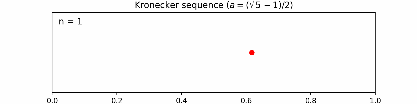
新しい点(赤)が毎回既存の点の間を埋めるように配置され、
Discrepancy と連分数展開
1次元の場合、
連分数展開とは、無理数
と表すものです。
Footnotes
-
Paskov, Spassimir H and Traub, Joseph F, Faster valuation of financial derivatives, The Journal of Portfolio Management Vol. 22, No. 1, pp. 113—120 (1995) ↩ ↩2
-
Matt Pharr and Wenzel Jakob and Greg Humphreys, Physically Based Rendering: From theory to implementation, Morgan Kaufmann (2016) ↩
-
Balandat, Maximilian and Karrer, Brian and Jiang, Daniel and Daulton, Samuel and Letham, Ben and Wilson, Andrew G and Bakshy, Eytan, BoTorch: A framework for efficient Monte-Carlo Bayesian optimization, Advances in neural information processing systems Vol. 33, pp. 21524—21538 (2020) ↩
-
Niederreiter, Harald, Random Number Generation and Quasi-Monte Carlo Methods, SIAM (1992) ↩ ↩2
-
Caflisch, Russel E, Monte Carlo and quasi-Monte Carlo methods, Acta Numerica Vol. 7, pp. 1—49 (1998) ↩ ↩2
-
Van der Corput, JG and Schaake, G, Ungleichungen für Polynome und trigonometrische Polynome, Compositio Mathematica Vol. 2, pp. 321—361 (1935) ↩
-
Halton, John H, On the efficiency of certain quasi-random sequences of points in evaluating multi-dimensional integrals, Numerische Mathematik Vol. 2, pp. 84—90 (1960) ↩
-
Bratley, Paul and Fox, Bennett L, Algorithm 659: Implementing Sobol’s quasirandom sequence generator, ACM Transactions on Mathematical Software (TOMS) Vol. 14, No. 1, pp. 88—100 (1988) ↩
-
Antonov Ilya A and Saleev VM, An economic method of computing LP
-sequences, USSR Computational Mathematics and Mathematical Physics Vol. 19, No. 1, pp. 252—256 (1979) ↩ ↩2